
Here is a utility I made for visualizing filters with Keras, using a few regularizations for more natural outputs.
You can use it to visualize filters, and inspect the filters as they are computed.
By default the utility uses the VGG16 model, but you can change that to something else.
The entire VGG16 model weights about 500mb.
However we don’t need to load the entire model if we only want to explore the the convolution filters and ignore the final fully connected layers.
You can download a much smaller model containing only the convolution layers (~50mb) from here:
https://github.com/awentzonline/keras-vgg-buddy
There is a lot of work being done about visualizing what deep learning networks learned.
This in part is due to criticism saying that it’s hard to understand what these black box networks learned, but this is also very useful to debug them.
Many techniques propagating gradients back to the input image became popular lately, like Google’s deep dream, or even the neural artistic style algorithm.
I found the Stanford cs231n course section to be good starting point for all this:
http://cs231n.github.io/understanding-cnn/
This awesome Keras blog post is a very good start for visualizing filters with Keras:
http://blog.keras.io/how-convolutional-neural-networks-see-the-world.html
The idea is quite simple: we want to find an input image that would produce the largest output from one of convolution filters in one of the layers.
To do that, we can perform back propagation from the output of the filter we’re interested in, back to an input image. That gives us the gradient of the output of the filter with respect to the input image pixels.
We can use that to perform gradient ascent, searching for the image pixels that maximize the output of the filter.
The output of the filter is an image. We need to define a scalar score function for computing the gradient of it with respect to the image.
One easy way of doing that, is just taking the average output of that filter.
If you look at the filters there, some look kind of noisy.
This project suggested using a combination of a few different regularizations for producing more nice looking visualizations, and I wanted to try those out.
No regularization
Lets first look at the visualization produced with gradient ascent for a few filters from the conv5_1 layer, without any regularizations:
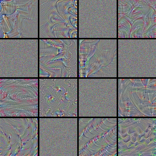
Some of the filters did not converge at all, and some have interesting patterns but are a bit noisy.
L2 decay
The first simple regularization they used in “Understanding Neural Networks Through Deep Visualization” is L2 decay.
The calculated image pixels are just multiplied by a constant < 1. This penalizes large values.
Here are the same filters again, using only L2 decay, multiplying the image pixels by 0.8:
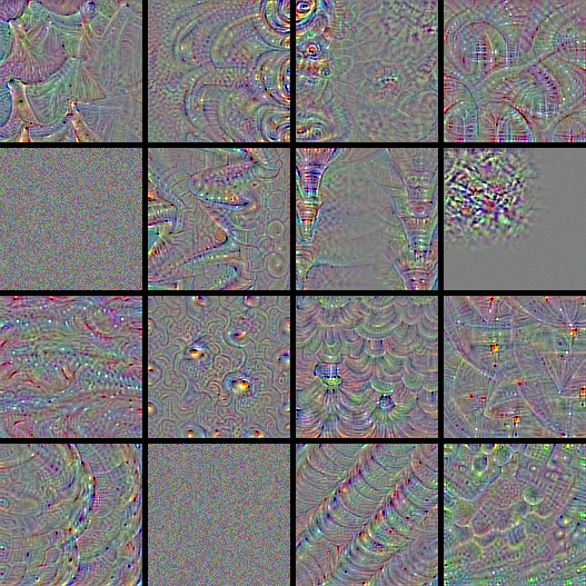
Notice how some of the filters contain more information, and a few of filters that previously did not converge now do.
Gaussian Blur
The next regularization just smooths the image with a gaussian blur.
In the paper above they apply it only once every few gradient ascent iterations, but here we apply it every iterations.
Here are the same filters, now using only gaussian blur with a 3x3 kernel:
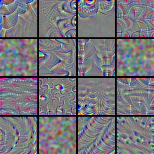
Notice how the structures become thicker, while the rest becomes smoother.
Removing pixels with small norms
This regularization zeros pixels that had weak gradient norms.
For each RGB channels the percentile of the average gradient value is
Even where a pattern doesn’t appear in the filters, pixels will have noisy non zero values.
By clipping weak gradients we can have more sparse outputs.
Gallery
Here are 256 filters with the Gaussian blur and L2 decay regularizations, and a small weight for the small norm regularization:
