Class activation maps in Keras

Class activation maps in Keras for visualizing where deep learning networks pay attention

Github project with all the code

Class activation maps are a simple technique to get the discriminative image regions used by a CNN to identify a specific class in the image.
In other words, a class activation map (CAM) lets us see which regions in the image were relevant to this class.
The authors of the paper show that this also allows re-using classifiers for getting good localization results, even when training without bounding box coordinates data.
This also shows how deep learning networks already have some kind of a built in attention mechanism.

This should be useful for debugging the decision process in classification networks.

To be able to create a CAM, the network architecture is restricted to have a global average pooling layer after the final convolutional layer, and then a linear (dense) layer.
Unfortunately this means we can’t apply this technique on existing networks that don’t have this structure. What we can do is modify existing networks and fine tune them to get this.
Designing network architectures to support tricks like CAM is like writing code in a way that makes it easier to debug.

The first building block for this is a layer called global average pooling.
After the last convolutional layer in a typical network like VGG16, we have an N-dimensional image, where N is the number of filters in this layer.
For example in VGG16, the last convolutional layer has 512 filters.
For an 1024x1024 input image (lets discard the fully connected layers, so we can use any input image size we want), the output shape of the last convolutional layer will be 512x64x64. Since 1024/64 = 16, we have a 16x16 spatial mapping resolution.
A global average pooling (GAP) layer just takes each of these 512 channels, and returns their spatial average.
Channels with high activations, will have high signals.
Lets look at keras code for this:

def global_average_pooling(x):
    return K.mean(x, axis = (2, 3))

def global_average_pooling_shape(input_shape):
    return input_shape[0:2]

The output shape of the convolutional layer will be [batch_size, number of filters, width, height].
So we can take the average in the width/height axes (2, 3).
We also need to specify the output shape from the layer, so Keras can do shape inference for the next layers. Since we are creating a custom layer here, Keras doesn’t really have a way to just deduce the output size by itself.

The second building block is to assign a weight to each output from the global average pooling layer, for each of the categories.
This can be done by adding a dense linear layer + softmax, training an SVM on the GAP output, or applying any other linear classifier on top of the GAP.
These weights set the importance of each of the convolutional layer outputs.

Lets combine these building blocks in Keras code:

def get_model():
    model = VGG16_convolutions()
    model = load_model_weights(model, "vgg16_weights.h5")

    model.add(Lambda(global_average_pooling, 
              output_shape=global_average_pooling_shape))
    model.add(Dense(2, activation = 'softmax', init='uniform'))
    sgd = SGD(lr=0.01, decay=1e-6, momentum=0.5, nesterov=True)
    model.compile(loss = 'categorical_crossentropy', optimizer = sgd, metrics=['accuracy'])
    return model

Now to create a heatmap for a class we can just take output images from the last convolutional layer, multiply them by their assigned weights (different weights for each class), and sum.

def visualize_class_activation_map(model_path, img_path, output_path):
    model = load_model(model_path)
    original_img = cv2.imread(img_path, 1)
    width, height, _ = original_img.shape

    #Reshape to the network input shape (3, w, h).
    img = np.array([np.transpose(np.float32(original_img), (2, 0, 1))])

    #Get the 512 input weights to the softmax.
    class_weights = model.layers[-1].get_weights()[0]
    final_conv_layer = get_output_layer(model, "conv5_3")
    get_output = K.function([model.layers[0].input], [final_conv_layer.output, 
    model.layers[-1].output])
    [conv_outputs, predictions] = get_output([img])
    conv_outputs = conv_outputs[0, :, :, :]

    #Create the class activation map.
    cam = np.zeros(dtype = np.float32, shape = conv_outputs.shape[1:3])
    class = 1
    for i, w in enumerate(class_weights[:, class]):
            cam += w * conv_outputs[i, :, :]

To test this out I trained a poor man’s person/not person classifier on person images from here:
http://pascal.inrialpes.fr/data/human
In the training all the images are resized to 68x128, and 20% of the images are used for validation.
After 11 epochs the model over-fits the training set with almost 100% accuracy, and gets about 95% accuracy on the validation set.

To speed up the training, I froze the weights of the VGG16 network (in Keras this is as simple as model.trainable=False), and trained only the weights applied on the GAP layer.
Since we discarded all the layers after the last convolutional layer in VGG16, we can load a much smaller model:
https://github.com/awentzonline/keras-vgg-buddy

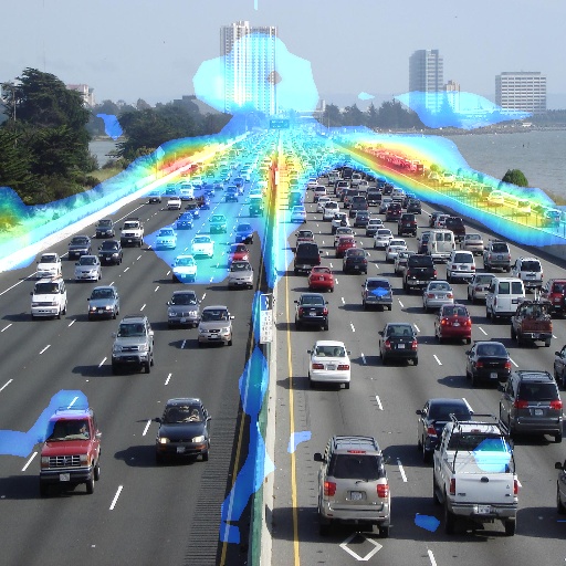
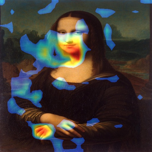
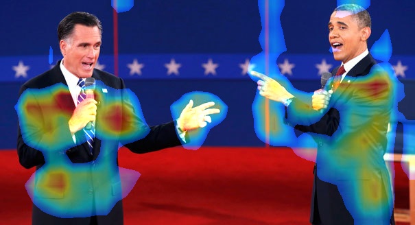
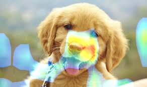
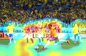
Here are some more examples, using the weights for the “person” category:

In this image it’s disappointing that the person classifier made a correct decision without even using the face regions at all.
Perhaps it should be trained on more images with clear faces.
Class activation maps look useful for understanding issues like this.

Here’s an example with weights from the “not person” category.
It looks like it’s using large “line-like” regions for making a “not person” decision.