A Computer Vision and Machine learning blog

My photo
I'm a Computer Vision and Machine learning developer.

Friday, April 24, 2015

Simple Image saliency detection from histogram backprojection

Image saliency detection is about identifying the interesting parts of an image, the parts of the image human eyes would fix on.
enter image description here enter image description here
Saliency detection is used in a lot of applications, the most popular of them is probably automatic thumbnail generation, where a descriptive thumbnail has to be generated for an image.
Usually a saliency map is generated, where a pixel is bright if it’s salient, and dark otherwise.
There are lots of interesting papers on this. Check out a great overview on saliency detection.
Anyway, in this post I’l share a simple heuristic for saliency detection.
The basic idea is that usually salient pixels should have very different colors than most of the other pixels in the image.
We measure each pixel’s similarity to the background by histogram back-projection.
Finally, we refine the saliency map with Grabcut.
So here we go.
Original image (taken at Mount. Takao, Japan)
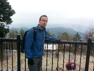
enter image description here

1. Preprocessing: Filter the image with Mean Shift for an initial soft segmentation of the image.

This groups together close pixels that are similar, and generates a very smooth version of the image.
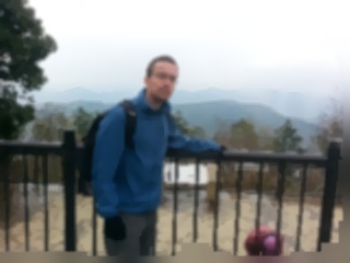
enter image description here
Some of the saliency papers call an inital segmentation stage - “abstraction”.
It’s common that each segment is compared somehow to other segments to give it a saliency score.
We won’t do that here, though.
For speed we use the multiscale pyramidal meanshift version in OpenCV.
This stage isn’t entirely necessary, but improves results on some images.
cv2.pyrMeanShiftFiltering(img, 2, 10, img, 4)

2. Back-project the Hue, Saturation histogram of the entire image, on the image itself.

The back-projection for each channel pixel is just the intensity, divided by how many pixels have that intensity.
It’s an attempt to assign each pixel a probability of belonging to the background.
We use only 2 bins for each channel.
That means we quantize the image into 4 colors (since we have 2 channels).
The more levels we use, the more details we get in the saliency map.
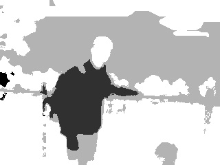
enter image description here
Notice how the blue jacket gets low values, since it’s unique and different from the background.
Also notice how the face back-projection is not unique.
That’s bad, we will try to fix that later.
def backproject(source, target, levels = 2, scale = 1):
    hsv = cv2.cvtColor(source,  cv2.COLOR_BGR2HSV)
    hsvt = cv2.cvtColor(target, cv2.COLOR_BGR2HSV)
    # calculating object histogram
    roihist = cv2.calcHist([hsv],[0, 1], None, [levels, levels], [0, 180, 0, 256] )

    # normalize histogram and apply backprojection
    cv2.normalize(roihist,roihist,0,255,cv2.NORM_MINMAX)
    dst = cv2.calcBackProject([hsvt],[0,1],roihist,[0,180,0,256], scale)
    return dst
backproj = np.uint8(backproject(img, img, levels = 2))

3. Process the back-projection to get a saliency map.

So here we smooth the back-projection image with mean shift, enhance the contrast of the saliency map with histogram equalization, and invert the image.
The goal is to produce a smooth saliency map where salient regions have bright pixels.
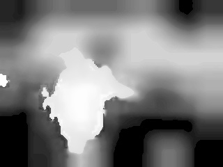
enter image description here
cv2.normalize(backproj,backproj,0,255,cv2.NORM_MINMAX)

saliencies = [backproj, backproj, backproj]
saliency = cv2.merge(saliencies)
cv2.pyrMeanShiftFiltering(saliency, 20, 200, saliency, 2)
saliency = cv2.cvtColor(saliency, cv2.COLOR_BGR2GRAY)
cv2.equalizeHist(saliency, saliency)

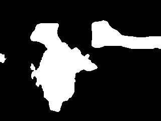
4. Threshold.
enter image description here
Ok, we have a few issues here:
- The segmentation is pretty rough.
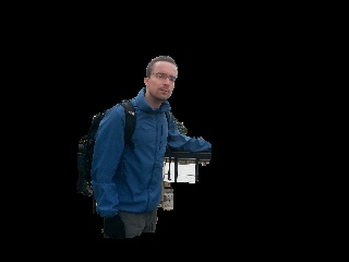
- My head isn’t attached to the salient region.
(T, saliency) = cv2.threshold(saliency, 200, 255, cv2.THRESH_BINARY)

5. Find the bounding box of the connected component with the largest area.

We now have two salient regions.
A heuristic we use here is that the salient object will probably be the largest one.
We could’ve similarly assumed that the salient object will usually be closest to the center.
Saliency papers call that “encoding a prior”, since we use prior knowledge about how salient objects look.
def largest_contour_rect(saliency):
    contours, hierarchy = cv2.findContours(saliency * 1,
    cv2.RETR_LIST,cv2.CHAIN_APPROX_SIMPLE)

    contours = sorted(contours, key = cv2.contourArea)
    return cv2.boundingRect(contours[-1])

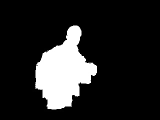
6. Refine the salient region with Grabcut.

We use the bounding box as an initial foreground estimation, and apply Grabcut.
This makes the salient region segmentation much more accurate,
and most importantly, attaches back my head.
enter image description hereenter image description hereenter image description here
def refine_saliency_with_grabcut(img, saliency):
    rect = largest_contours_rect(saliency)
    bgdmodel = np.zeros((1, 65),np.float64)
    fgdmodel = np.zeros((1, 65),np.float64)
    saliency[np.where(saliency > 0)] = cv2.GC_FGD
    mask = saliency
    cv2.grabCut(img, mask, rect, bgdmodel, fgdmodel, 1, cv2.GC_INIT_WITH_RECT)
    mask = np.where((mask==2)|(mask==0),0,1).astype('uint8')
    return mask
Link to the code on github.
I like this method since it’s simple, but it has it’s drawbacks.
enter image description hereenter image description here

Friday, December 5, 2014

Image Fisher Vector In Python

Although the state of the art in image classification is deep learning,
Bag of words approaches still perform well on many image datasets.

Fisher vectors is the state of the art in that approach, allowing training more discriminative classifiers with a lower vocabulary size.

I wrote a simple Python implementation for calculating fisher vectors and using it to classify image categories:

You might want to look here for a derivation: 

The main improvement here is extracting a richer feature vector from images compared to bag of words.

In Bag of Words, for each local feature we find the closest word in the vocabulary, and add +1 to the histogram of the vocabulary in the input image.
But we could have sampled more data: 
- How far is each feature from its closest vocabulary word.
- How far is the feature from other vocabulary words.
- The distribution of the vocabulary words themselves. 

Brief outline of fisher vectors

Vocabulary learning with GMM:
- Sample many features from input images.
- Fit a Gaussian Mixture Model on those features. 
- The result is a vocabulary of dominant features in the image, and their distributions.

Image representation based on the vocabulary:
- Measure the expectation of the difference and distance of the image features, from each Gaussian distrubution, using the likelihood a feature belongs to certain gaussian. 
- Concatenate the resulting vector for each vocabulary word, into one large descriptor vector.

There is also a normalization step that I will skip here but is a part of the implementation, that is important if the features are fed into a classifier like SVM that needs normalized inputs.

This is a generalization of bag of words. If you set the likelihood of a feature to a vocabulary word to be 1 to it's closest word and 0 to the rest, 
and if you redefine the distance to be a constant "1", you get the original bag of words model.

Trying out the implementation:
python fisher.py <path_to_image_directory> <vocabulary size>
The image directory should contain two sub folders, one for the images of each class.

It currently just trains a model and then classifies the images.
The input images definitely need to be partitioned into training and validation parts.

One more thing:
Fisher vectors are successfully used in image recognition, check out:
http://www.robots.ox.ac.uk/~vgg/publications/2013/Simonyan13/extras/simonyan13_ext.pdf
In their paper they extract features densely from a grid,  reduce the dimensionality with PCA, and augment the features with their spacial location.

Monday, May 5, 2014

Bag Of Visual Words model for image classification

I wanted to play around with Bag Of Words for visual classification, so I coded a Matlab implementation that uses VLFEAT for the features and clustering.
It was tested on classifying Mac/Windows desktop screenshots.


For a small testing data set (about 50 images for each category), the best vocabulary size was about 80.
It scored 97% accuracy on the training set, and 85% accuracy on the cross validation set,
so the over-fitting can be improved a bit more.

Overview:

1. Collect a data set of examples. I used a python script to download images from Google.
2. Partition the data set into a training set, and a cross validation set (80% - 20%).
3. Find key points in each image, using SIFT.
4. Take a patch around each key point, and calculate it's Histogram of Oriented Gradients (HoG). Gather all these features.
5. Build a visual vocabulary by finding representatives of the gathered features (quantization).
This done by k-means clustering.
6. Find the distribution of the vocabulary in each image in the training set.
This is done by a histogram with a bin for each vocabulary word.
The histogram values can be either hard values, or soft values.
Hard values means that for each descriptor of a key point patch in an image, we add 1 to the bin of the vocabulary word closest to it in absolute square value.
Soft values means that each patch votes to all histogram bins, but give a higher weight to bin representing words that are similar to that patch. Take a look here.
7. Train an SVM on the resulting histograms (each histogram is a feature vector, with a label).
8. Test the classifier on the cross validation set.
9. If results are not satisfactory, repeat 5 for a different vocabulary size and a different SVM parameters.

Visualization of the vocabulary learned by the clustering


Source Code

https://github.com/jacobgil/BagOfVisualWords

Wednesday, April 16, 2014

Refining the Hough Transform with CAMSHIFT

The Circular Hough Transform result is often not very accurate due to noise\details\occlusions.
Typical ways of dealing with this are:
1. Hand tuning the Hough Transform parameters.
2. Pre-processing the image aggressively before the transform is applied.

One trick I use to fix the circles positions is an iterative search in windows around the initial circles, I hope to have a future post about this here.

But now I will share a much simpler strategy that works well in some cases: Use CAMSHIFT to track the circular object in a window around the initial circles positions.

The idea is that the initial circle center position area holds information about how the circular object looks like, for example its color distribution. This is complementary to the Hough transform that uses only spatial information (the binary votes in the Hough space).

The steps:

  1. Find circles with the Circular Hough Transform.
  2. Find the histogram inside a small box around each circle. In a more general case we can use any kind of features we like, like texture features or something, but here we will stick with color features.
  3. For each pixel, find the probability it belongs to the circular object (back-projection).
  4. Optional: apply some strategy to fill holes in the back-projection image caused by occlusions. We can use morphology operations like dilating for example.
  5. Use CAMSHIFT to track the the circular object starting in a window around the initial circle position.


Conveniently for us, CAMSHIFT is included in OpenCV!

I encourage you to read the original CAMSHIFT paper to learn more about it:
Computer Vision Face Tracking For Use in a Perceptual User
Interface
Gary R. Bradski, Microcomputer Research Lab, Santa Clara, CA, Intel Corporation
Link to the paper

Code (C++, using OpenCV):
#include "opencv2/highgui/highgui.hpp"
#include "opencv2/imgproc/imgproc.hpp"
#include "opencv2/core/core.hpp"
#include "opencv2/video/tracking.hpp"
#include <tuple>

using namespace cv;
using namespace std;

//This is used to obtain a window inside the image,
//and cut it around the image borders.
Rect GetROI(Size const imageSize, Point const center, int windowSize)
{
    Point topLeft (center.x - windowSize / 2, center.y - windowSize / 2);

     if (topLeft.x + windowSize > imageSize.width || topLeft.y + windowSize >
         imageSize.height)
    {
         windowSize = 
         min(imageSize.width - topLeft.x, imageSize.height - topLeft.y);
    } 
    return Rect(topLeft.x, topLeft.y, windowSize, windowSize);
}

//This is used to find pixels that likely belong to the circular object
//we wish to track.
Mat HistogramBackProjectionForTracking(Mat const& image, Rect const window)
{
     const int sizes[] = {256,256,256};
     float rRange[] = {0,255};
     float gRange[] = {0,255};
     float bRange[] = {0,255};
     const float *ranges[] = {rRange,gRange,bRange};
     const int channels[] = {0, 1, 2};

     Mat roi = image(window);

     Mat hist;
     if (image.channels() == 3)
      calcHist(&roi, 1, channels, Mat(), hist, 3, sizes, ranges);
     else
      calcHist(&roi, 1, &channels[0], Mat(), hist, 1, &sizes[0], &ranges[0]);

     Mat backproj;
     calcBackProject(&image, 1, channels, hist, backproj, ranges);
     return backproj;
}

//Return a new circle by using CAMSHIFT to track the object around the initial circle.
tuple<Point, int> HoughShift(Point const center, int const radius, Mat const& image)
{
    Mat backproj = HistogramBackProjectionForTracking(image, 
    GetROI(image.size(),center, radius));

     //Fill holes:
     cv::dilate(backproj, backproj, cv::Mat(), cv::Point(-1,-1));
     cv::dilate(backproj, backproj, cv::Mat(), cv::Point(-1,-1));

    const int windowTrackingSize = 4 * radius;
    RotatedRect track = CamShift(backproj, GetROI(image.size(), center,
    TermCriteria( CV_TERMCRIT_EPS | CV_TERMCRIT_ITER, 10, 1 ));

    return make_tuple(track.center, (track.size.width + track.size.height )/ 4);
}

int main(int argc, char** argv)
{
     Mat image = cv::imread("image.jpg");

     Mat before, after; image.copyTo(before); image.copyTo(after);
     Mat gray; cv::cvtColor(image, gray, CV_BGR2GRAY);

     std::vector<cv::Vec3f> circles;
     HoughCircles(gray, circles, CV_HOUGH_GRADIENT, 2, gray.cols / 3, 20, 40,
     gray.cols / 20, gray.cols / 5);

     for (int i = 0; i < circles.size(); ++i)
     {
         auto circle = HoughShift(Point(circles[i][0], circles[i][1]), 
         circles[i][2], image);

         circle(before, Point(circles[i][0], circles[i][1]), circles[i][2], 
         Scalar(128, 128, 30),  2);
         circle(after, get<0>(circle), get<1>(circle), Scalar(255, 0 , 0), 2);
     }

     imshow("Initial Circles", before);
     imshow("Refined Circles", after);
     waitKey(-1);

     return 0;
}